
Compression Method
The JPG Format is very complex. I'll repeat the same information in Three different ways.
Outline, Text, Detailed.
Outline
The JPG Format uses multiple methods of compression
1. Color Space Conversion, and chrominance reduction
2. High frequency information reduction
3. RLE (Run Length Encoding)
4. Huffman coding (Similar to the Index and LZW methods)
Text
The Following printed without permission from "www.Desinger-info.com"
"What made the JPEG completely different was the acceptance that its compression could be "lossy", that is that information could be thrown away. Of course the trick was to make this loss as imperceptible as possible and the result was a five-stage process. To begin with the image is converted to a color space (LAB again) where color and luminance are handled separately. The two chrominance channels are then downsampled as the eye is not as attuned to changes in color as to changes in brightness. In this way pixel data can be cut by 50% with almost no perceived loss of quality. Next the image is broken into 8x8 tiles that are transformed through a Discrete Cosine Transformation (DCT) into a matrix that separates the high frequency information from the low frequency information. The high frequency information can then again be discarded without the eye noticing. Each block is then quantized according to the user-set, 1-100 quality setting. Finally the resulting co-efficients are losslessly compressed using Huffman compression. The end result is a compression ratio of up to 25:1 with very little perceived loss of quality on continuous tone files."
Detailed
1. Color Space Conversion, and chrominance reduction
"What made the JPEG completely different was the acceptance that its compression could be "lossy", that is that information could be thrown away. Of course the trick was to make this loss as imperceptible as possible and the result was a five-stage process."
Read the section on "File compression and Data Loss" if you need further information. File compression. Many of the ideas involve the same issues of color reduction as the GIF format. Multiple shades of the same color are averaged, and fewer unique colors are used for the image as a whole. As a side note, the MP3 Audio format is very, very, similar.
"To begin with the image is converted to a color space (LAB again) where color and luminance are handled separately."
See the support article Color space if you need information about color spaces on the computer.
"The two chrominance channels are then downsampled as the eye is not as attuned to changes in color as to changes in brightness. In this way pixel data can be cut by 50% with almost no perceived loss of quality."
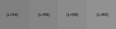
Brightness vs Color Perception
How about an example?
The jpg compression format does most of it's work, on small 8 pixel by 8 pixel sections of the image. Each of these pixels have an R, a G, and a B number for color. Because this is alot to type out, and is really hard to view, Let's use a graphic. Below is an 8x8 matrix of RGB colors that represents an 8x8 matrix of RGB numbers.
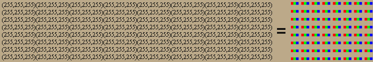
First, we convert all of the colors to their LAB colorspace equivalent.
Note: Remember that LAB is L(Luminance), a(Green to Red), b(Yellow to Blue).
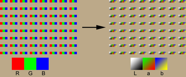
Next, we separate out the L, a, and b components into their own separate matrixes so that we can work on the Luminance and color components separately.
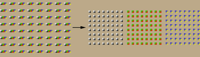
Next, we will group the 'a' and 'b' colors into 2x2 pixel groups. We will then take the average color of the 2x2 pixel group and use this value for all 4 pixels.
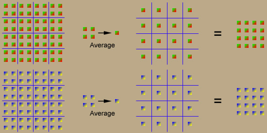
And here is our before and after comparison
And a (192/96) or 50% Reduction in space.
Note: Most of this was developed for use in TV broadcasting. To fit more TV channels on the air they needed a method to shrink the bandwidth.
Note: The decision as to whether and when to use chroma down-sampling is optional. It is dependent on the particular JPEG implementation. In Adobe Photoshop 5, this feature is turned off for quality 5 and above.
2. High frequency information reduction
"Next the image is broken into 8x8 tiles that are transformed through a Discrete Cosine Transformation (DCT) into a matrix that separates the high frequency information from the low frequency information. The high frequency information can then again be discarded without the eye noticing."
Note: While we have averaged the color information for each 2x2 area, we still work with the color data in 8x8 pixel sections. It simply means that we have many duplicate entries. From the unique nature of the next steps, we will still see a reduction in file size because of the color reduction.
2a. Discrete Cosine Transformation
The "Discrete Cosine Transformation" is a calculus formula that is applied to each value one at a time. It is a matrix math function, which means after using the formula you have another 8x8 matrix of numbers. This formula is magic. Somehow you change from a 8x8 matrix of RGB colors to a new matrix that shows higher frequencies in the lower right and lower frequencies in the upper left.
And for those of you who remember computers better than calculus, here's some code.
This would be an example of what you would have after this step. You would have 3 of these matrixes, one for L, a, and b.
Once again the purpose is to quantize(round) values that the human eye are less sensitive to. Just to confuse the issue, they use the term "Quantization Matrix" to describe this. This part is actually very simple. When the JPG standard was developed tests were done to determine what frequencies the human eye was sensitive to. Then they chose rounding ranges. Say numbers from 100-120 would be 110, and numbers 10-12 would be 11. These ranges are not equal because the human eye is more sensitive to lower frequencies.
"Each block is then quantized according to the user-set, 1-100 quality setting."
The amount that you round is the quality value when saving JPG Files. If you round alot, you will have poor quality, and if you only round alittle you will have good quality. Note that the idiots at Adobe photoshop decided to give you values of compression between 1-12 when saving JPG files. Arggggh! You can get around this by using the "save for web" option which will let you save with quality settings from 1-100.
Lets Look at an example.
Note: For greater amounts of compression you could multiply each number in the quantization table by a constant. This would result in a much greater amount of rounding. This constant is the quality factor.
Note: The values in the quantization table are SUBJECTIVE. There are no 'right' and no 'wrong' values. The values are actually stored inside each jpg file when the file is saved. This means that you can use whatever table you wish, and anyone can still read the file. This is another reason why when you save a jpg file in two different programs, and you use the same settings, the files look slightly different.
3. RLE (Run Length Encoding)
*The description misses a Step here so I'll add it
"The resulting matrix is then RLE encoded."
What is not apparent by reading this description is large amount of rounding that is done to the numbers in the 8x8 matrix. For example, here is an un-quantized and quantized matrix
Notice how reading the matrix in a zig-zag pattern the last 44 numbers are zero. This greatly enhances the compression.
4. Huffman coding (Similar to the Winzip and LZW methods)
"Finally the resulting co-efficient are losslessly compressed using Huffman compression."
And just for the hell of it, the final file is compressed the same as the winzip file format ,,,, Just in case.
And if you fully understand this,,,,, that makes one of us.
Important Points
The compression is "lossy". Data is rounded to save space.
The amount of compression is variable and controlled by the person who saves the file.
The Compression is applied in 8x8 pixel groups. Quality problems with the final image will will follow the borders of these 8x8 pixel groups. Sometimes these are called block artifacts.
Next -----> Examples and Comments
The JPG Format is very complex. I'll repeat the same information in Three different ways.
Outline, Text, Detailed.
Outline
The JPG Format uses multiple methods of compression
1. Color Space Conversion, and chrominance reduction
2. High frequency information reduction
3. RLE (Run Length Encoding)
4. Huffman coding (Similar to the Index and LZW methods)
Text
The Following printed without permission from "www.Desinger-info.com"
"What made the JPEG completely different was the acceptance that its compression could be "lossy", that is that information could be thrown away. Of course the trick was to make this loss as imperceptible as possible and the result was a five-stage process. To begin with the image is converted to a color space (LAB again) where color and luminance are handled separately. The two chrominance channels are then downsampled as the eye is not as attuned to changes in color as to changes in brightness. In this way pixel data can be cut by 50% with almost no perceived loss of quality. Next the image is broken into 8x8 tiles that are transformed through a Discrete Cosine Transformation (DCT) into a matrix that separates the high frequency information from the low frequency information. The high frequency information can then again be discarded without the eye noticing. Each block is then quantized according to the user-set, 1-100 quality setting. Finally the resulting co-efficients are losslessly compressed using Huffman compression. The end result is a compression ratio of up to 25:1 with very little perceived loss of quality on continuous tone files."
Detailed
1. Color Space Conversion, and chrominance reduction
"What made the JPEG completely different was the acceptance that its compression could be "lossy", that is that information could be thrown away. Of course the trick was to make this loss as imperceptible as possible and the result was a five-stage process."
Read the section on "File compression and Data Loss" if you need further information. File compression. Many of the ideas involve the same issues of color reduction as the GIF format. Multiple shades of the same color are averaged, and fewer unique colors are used for the image as a whole. As a side note, the MP3 Audio format is very, very, similar.
"To begin with the image is converted to a color space (LAB again) where color and luminance are handled separately."
See the support article Color space if you need information about color spaces on the computer.
"The two chrominance channels are then downsampled as the eye is not as attuned to changes in color as to changes in brightness. In this way pixel data can be cut by 50% with almost no perceived loss of quality."
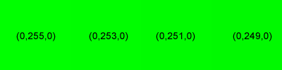  |
The Image on the Top is comprised of 4 sample colors. Each sample color has
a green value that is 2 greater than the one beside it. Notice how subtle
this variation is. The Image on the bottom is also comprised of 4 sample colors. Each of these samples has a brightness(L) that is 2 greater that the one beside it. Notice how much more pronounced this difference is. |
How about an example?
The jpg compression format does most of it's work, on small 8 pixel by 8 pixel sections of the image. Each of these pixels have an R, a G, and a B number for color. Because this is alot to type out, and is really hard to view, Let's use a graphic. Below is an 8x8 matrix of RGB colors that represents an 8x8 matrix of RGB numbers.
First, we convert all of the colors to their LAB colorspace equivalent.
Note: Remember that LAB is L(Luminance), a(Green to Red), b(Yellow to Blue).
Next, we separate out the L, a, and b components into their own separate matrixes so that we can work on the Luminance and color components separately.
Next, we will group the 'a' and 'b' colors into 2x2 pixel groups. We will then take the average color of the 2x2 pixel group and use this value for all 4 pixels.
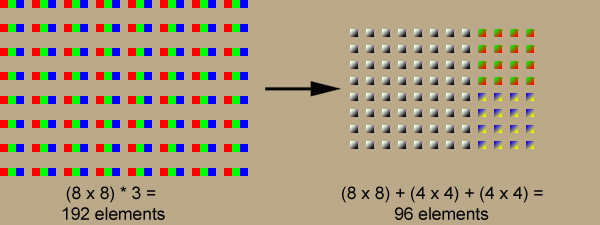
And here is our before and after comparison
And a (192/96) or 50% Reduction in space.
Note: Most of this was developed for use in TV broadcasting. To fit more TV channels on the air they needed a method to shrink the bandwidth.
Note: The decision as to whether and when to use chroma down-sampling is optional. It is dependent on the particular JPEG implementation. In Adobe Photoshop 5, this feature is turned off for quality 5 and above.
2. High frequency information reduction
"Next the image is broken into 8x8 tiles that are transformed through a Discrete Cosine Transformation (DCT) into a matrix that separates the high frequency information from the low frequency information. The high frequency information can then again be discarded without the eye noticing."
Note: While we have averaged the color information for each 2x2 area, we still work with the color data in 8x8 pixel sections. It simply means that we have many duplicate entries. From the unique nature of the next steps, we will still see a reduction in file size because of the color reduction.
2a. Discrete Cosine Transformation
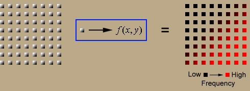
The "Discrete Cosine Transformation" is a calculus formula that is applied to each value one at a time. It is a matrix math function, which means after using the formula you have another 8x8 matrix of numbers. This formula is magic. Somehow you change from a 8x8 matrix of RGB colors to a new matrix that shows higher frequencies in the lower right and lower frequencies in the upper left.
And for those of you who remember computers better than calculus, here's some code.
----------------------------
for u = 0 to 7
	for v = 0 to 7
		F(u,v) = Getdct(u,v,OriginalMatrix);
	end
end

Function Getdct(u,v,OriginalMatrix)
for x = 0 to 7
  for y = 0 to 7
    sum = sum + ( OriginalMatrix(x,y)
                  * cos( (((2*x)+1) * u *pi )/16)
                  * cos( (((2*y)+1) * v * pi)/16) );
  end
end
----------------------------
And for those of you who want this as a graphic. For each number in the
matrix you will put it into the DCT calculus formula. You will be left
with another 8x8 matrix of numbers that is ordered by frequency.This would be an example of what you would have after this step. You would have 3 of these matrixes, one for L, a, and b.
	217  32  15  16   1  21   7   2
	 15   5   3   3   8   1   4  11
	 22   8  13   6   6  13   0   0
	 23  25  20 112   5   3   7  10
	 12   5   5   5   7  21  30  13
	 15   9  27  27   9   7   5  15
	 10   7   5  29  17  19  24  11
	 13   6   6   2  21   1  15  17
2b. Quantize
Once again the purpose is to quantize(round) values that the human eye are less sensitive to. Just to confuse the issue, they use the term "Quantization Matrix" to describe this. This part is actually very simple. When the JPG standard was developed tests were done to determine what frequencies the human eye was sensitive to. Then they chose rounding ranges. Say numbers from 100-120 would be 110, and numbers 10-12 would be 11. These ranges are not equal because the human eye is more sensitive to lower frequencies.
"Each block is then quantized according to the user-set, 1-100 quality setting."
The amount that you round is the quality value when saving JPG Files. If you round alot, you will have poor quality, and if you only round alittle you will have good quality. Note that the idiots at Adobe photoshop decided to give you values of compression between 1-12 when saving JPG files. Arggggh! You can get around this by using the "save for web" option which will let you save with quality settings from 1-100.
Lets Look at an example.
	217  32  15  16   1  21   7   2         8   6   6   7   6   5   8   7
	 15   5   3   3   8   1   4  11         7   7   9   9   8  10  12  20
	 22   8  13   6   6  13   0   0        13  12  11  11  12  25  18  19
	 23  25  20 112   5   3   7  10        15  20  29  26  31  30  29  26
	 12   5   5   5   7  21  30  13        28  28  32  36  46  39  32  34
	 15   9  27  27   9   7   5  15        44  35  28  28  40  55  41  44
	 10   7   5  29  17  19  24  11        48  49  52  52  52  31  39  57
	 13   6   6   2  21   1  15  17        61  56  50  60  46  51  52  50

                  Matrix                        Quantization Table
For each number in the Matrix DIVIDE by the number in the Quantization table. Then Round Down.
217 / 8 = 27.1 = 27
 32 / 6 =  5.3 = 5
 15 / 6 =  2.5 = 2
 16 / 7 =  2.2 = 2
  1 / 6 =  0.2 = 0
 21 / 5 =  4.2 = 4
  7 / 8 =  0.9 = 0
  2 / 7 =  0.3 = 0

 27   5   2   2   0   4   0   0
  2   0   0   0   0   0   0   0
  1   0   1   0   0   0   0   0
  1   1   0   0   0   0   0   0
  0   0   0   0   0   0   0   0
  0   0   0   0   0   0   0   0
  0   0   0   0   0   0   0   0
  0   0   0   0   0   0   0   0

         Resulting Matrix
Note: This is the main step where data loss happens.Note: For greater amounts of compression you could multiply each number in the quantization table by a constant. This would result in a much greater amount of rounding. This constant is the quality factor.
Note: The values in the quantization table are SUBJECTIVE. There are no 'right' and no 'wrong' values. The values are actually stored inside each jpg file when the file is saved. This means that you can use whatever table you wish, and anyone can still read the file. This is another reason why when you save a jpg file in two different programs, and you use the same settings, the files look slightly different.
3. RLE (Run Length Encoding)
*The description misses a Step here so I'll add it
"The resulting matrix is then RLE encoded."
What is not apparent by reading this description is large amount of rounding that is done to the numbers in the 8x8 matrix. For example, here is an un-quantized and quantized matrix
 8   6   6   7   6   5   8   7         27   5   2   2   0   4   0   0
 7   7   9   9   8  10  12  20          2   0   0   0   0   0   0   0
13  12  11  11  12  25  18  19          1   0   1   0   0   0   0   0
15  20  29  26  31  30  29  26          1   1   0   0   0   0   0   0
28  28  32  36  46  39  32  34          0   0   0   0   0   0   0   0
44  35  28  28  40  55  41  44          0   0   0   0   0   0   0   0
48  49  52  52  52  31  39  57          0   0   0   0   0   0   0   0
61  56  50  60  46  51  52  50          0   0   0   0   0   0   0   0
As you can now see, most of the values will be zero. This can now be compressed by the same methods as the BMP RLE compression. Of note, just to be confusing the matrix is actually read in a diagonal zig-zag pattern to absolutely maximize the compression.
Notice how reading the matrix in a zig-zag pattern the last 44 numbers are zero. This greatly enhances the compression.
4. Huffman coding (Similar to the Winzip and LZW methods)
"Finally the resulting co-efficient are losslessly compressed using Huffman compression."
And just for the hell of it, the final file is compressed the same as the winzip file format ,,,, Just in case.
And if you fully understand this,,,,, that makes one of us.
Important Points
The compression is "lossy". Data is rounded to save space.
The amount of compression is variable and controlled by the person who saves the file.
The Compression is applied in 8x8 pixel groups. Quality problems with the final image will will follow the borders of these 8x8 pixel groups. Sometimes these are called block artifacts.
Next -----> Examples and Comments